In brief:
A program which graphically shows the behaviour of the pendulum, allows setting of several parameters and logs data for later analysis.
The program runs 24 / 7 on an older laptop with Linux Mint 21.
There is also an Analysing program which shows the data from the logfiles graphically.
You can download the complete code package.
The program is written in FreePascal with the Lazarus IDE. Lazarus / FPC is a complete development package for programs with a graphical user interface (GUI). It is freeware, living and available for many platforms a.o. Linux, Mack, Window$, Raspberry-Pi, Android.
I can give some support for the source code I provide here, but not for the development environment(s)
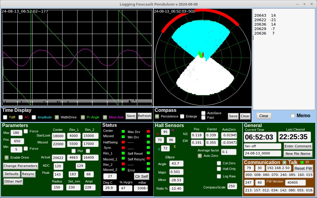
Fig 1. Dashboard.
From Top-Left to Bottom-Right:
Time display 500 x 360 px. Has two timescales. Slow: 5hr / div, Fast: 1px / halfswing = ca 100 sec / div.
New data arrives at the right side.
Below are some screenshots with explanation.
The checkboxes below the display allow turning on or off the traces.
The Save button produces a screenshot of the display like the ones below.
Compass display:
Right = East = 0°, over North increasing to 180° as usual in math.
Shows in real time the movement of the pendulum, as measured with the Hall sensors.
With the checkbox "Persistence" checked the dots will stay until the display is cleared. The time of Last Clear is displayed on the right in the "General" box. Here it is 8:28 ago, so we see around 1/4 of the foucault precession..
"Enlarge" scales the display 10 times more sensitive, and is used for precisely zeroing the TopMount.
"Autosave" produces a screenshot of the compass display every 5 minutes.
"Fast" makes a screenshot every 10 seconds for more detailed analysis.
We mark one halfswing as the first half (cyan) and the other halfswing as second (white). As there is no way to distinguish between these halfswings we name one number 1 and the other number 2, and count 1-2, 1-2, 1-2 etc. and try not to lose counts. This way we can also distiguish between the first and the second half of the Foucault rotation, indicated by the red circles on the perimeter.
On the Results page an animation of 1 complete Foucault cycle can be seen.
The memo box can list the Center Pass time at each zero crossing, and the difference with the previous passtime. This is used to center the floorplate with the coil set.
Parameters to be set:
Maximum an minimum width of the drive pulse, and the center position.
"Enable Drive" directly enables or disables the Drive Pulse.
"Force" boxes force the dive width, bypassing the mechanism for amplitude stabilisation.
For the Center, Rim 1 and Rim2 pass times we have settings for when to start looking for it and a time-out for when a passage is missed.
Reason: The Drive Pulse will induce a voltage in the other coils which may trigger a false reading.
"Change Parameters" sends (new) settings to the Arduino unit and also logs these settings in the Event Log file. The Arduino stores the parameters in EEPROM and reads them at startup.
"Defaults" sets the default values for these parameters.
"Resync" starts a synchronisation procedure in the Arduino software.
"Other half" switches the 1-2, 1-2, 1-2 countinge to the other half period of the pendulum. Note that we basically cannot distinguish between the two halves.
"Radius' is the diameter of the Rim coil.
"Set_mm" is the setpoint for the amplitude control system in mm.
"Ampl" gives the actual amplitude in mm.
Status:
Displays a number of situations.
"Clr Self" clears indications when the Arduino did a resync or system reset.
Temperature, relative Hygro and Barometric pressure as measred with a BME280 device.
The field above the word "Deg C" gives the temperature measured in the top unit.
Hall Sensors:
The actual readings from the Hall sensors in A/D converter values (8 bit conversions)
The North-South and East-West positions and farest positions found, and the Auto zero corrections
The ellipse parameters calculated.
Enable/disable AutoZero and an average factor for autozero.
Some option checkboxes for calibration and logging.
General:
Current time and last time the Compass display was cleared.
A possibility to enter a comment into the logfile.
The name of the logfile. Automatically changes at midnight time.
Communication:
This box gives info about the ethernet communication between the GUI and the Arduino.
Some screenshots from the Time Display.
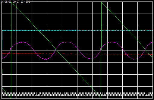
Fig 2.
Purple (5 hr / div) the length of the ellipse's minort axis x10 exaggerated. Midscale = zero, positive = CCW, negative = CW.
Green ((5 hr / div) the angle of the pendulum's swinging plane.
White (50 halfswings / div) the drive time minimum or maximum
Red (50 halfswings / div) the peak amplitude of the Center Pass signal, just before the center crossing. This signal is proportional with the velocity of the pendulum, it is strongly dependent on the height of the bob, and it becomes smaller when a more elliptical path develops.
Cyan the amplitude as calculated from the Rim fly-over time, and used for the amplitude stabilisation.
The scale is + / - 180 for signals with zero midscale, and 0 .. 320 for the other signals.
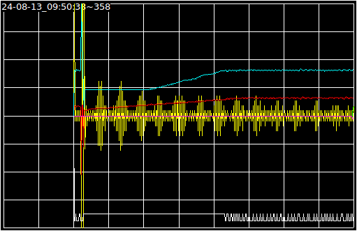
Fig 3.
This screenshot was taken a few minutes after a manual relaunch.
In yellow the difference in zero-crossing time of successive half swings.
Midscale = zero. Vetical: 100 usec / px gives 4.5 ms / div. As the bob's velocity in the center is 0.347 m/s this corresponds to 1.6 mm/div.
This signal is primarely used to center the coil assembly on the Floor Unit.
Here the coil set was well centered but we see a periodic change, caused by a small axial rotation of the bob, accidently introduced by the manual relaunch. This rotation has a period of ca. 50 sec, and dies out after some time.
Cyan: the amplitude as measured from the rim coil passege times. During the first 200 seconds the rim passes were missed, so there was no reliable reading. After the rimcoil passes were detected again we see the amplitude increase to the stabilisation level of 230 mm.
Red: the amplitude of the signal from the Center cross coil. We see an increase with the amplitude.
White: maximum or minimum width of the drive pulse. We see the maximum level until the stabilisation point has been reached. The the switching between min and max starts.
More screenshots on the Results page.
About the operation of the program
The operation of the program is quite self-explaining by name-giving and comments in the code.
The way the ellipse parameters are calculated needs some more explanation.
The coordinates of the Bob are derived from the Hall sensor signals by the formula Ypos = (North - South) / (North + South). For East - West the same recipe. This formula assumes a good linearity which of coarse is not there, but the results appear quite acceptable.
To determine the parameters of the ellipse I follow a number of steps. See drawing.
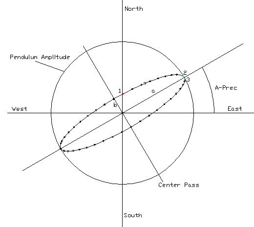
Fig. 4. Illustrates the process of finding the ellipse parameters.
For this example we have a clockwise rotating ellipse (see arrow in Q1) with a precession angle A-Prec w.r.t. the X-axis (EW) The long axis is labeled a, the short axis is b.
The dots represent the sampled positions of the Bob’s path. from messages appox. 10 times per second)
The moment where the Bob makes a Center Pass or a Rim pass is indicated in the first message after such an event.
Finding the end of the major axis is done by finding the sample laying the farest away from the center. For that we start at the moment of the Center Pass and track the absolute distances of the samples using Pythagoras’ law. When we find the first sample which is not further away than the previous one (3) we know that the previous one (2) was the farest away. Using the arctan2 function we find the Precession Angle.
Knowing that the precession angle wiil vary very slowly and that our samples are contaminated with noise we apply a walking averaging over many pendulum swings using the so called “leaking bucket” method where:
NewAverage = OldAverage * (1-f) + NewValue * f, where f is a value 0 < f < 1.
A
small fraction f gives a slow walking average, f near 1 gives a fast response.
The
next step is to determine the length of the minor axis of the ellipse.
For
that we take the first sample after the Center Pass. Its distance
from the center gives a good approximation of the length of the minort
axis.
We
also want to know the rotational direction of the ellipse. For that
we rotate the found sample over minus the earlier found
PrecessionAngle. The sample is now so to say on the ellipse when it
is laying with the major axis horizontally. The Y-polarity of the
sample now gives us the direction of the elliptical path. If it is
positive we have a CW rotation, if negative it is CCW.
To
calibrate the minor axis in mm we rely on the knowledge that the major
axis (= Pendulum Amplitude) is kept stable by the amplitude control
mechanism, in our case 230 mm. So we can easily find a calibration
factor for the minor axis, using the distance of the farest sample in
“Hall units”.
If
we would do these calculations for each halfswing we would find
opposite values for nearly everything and averages would approach
zero. That wo’nt work, so we do the calculations only for each
other halfswing. This means we must be sure that no Halfswing info is
missed. Normally this wo’nt happen, but for the case it does we
have a button to switch to the other halfswing.
From end 2023 I also try to use a different method of determining the ellipse parameters. I call it the Fourier method because it is in fact a spectrum analysis on one single frequency. One may also call it the Quadrature Method because it measures the amplitude and phase of the X- and Y movements of the pendulum.
The advantage of this method is that it uses all af the Hall data, where the current method uses only two points from the dataset and so produces more noisy results.
About stabilizing the amplitude. This is implemented in the Arduino Firmware. The GUI only sets the parameters for the control mechanism.
If the measured amplitude is lower than the setpoint, the width of the drive pulse is set to the value in the box "Max". If it is higher it will be the value in the "Min" box.
One should play a bit with the Upper and Lower values for on average equal times Maximal and Minimal as can be seen in the white trace on the timer display.
When the GUI stops working the Arduino will keep the Bob running, only no data are logged anymore.
The Analysing program reads one or more logfiles and presents the data in graphical format.
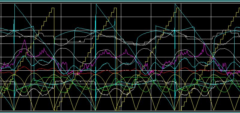
Fig 5. Output of the Analyse program with all taces on.
Individual traces can be switched on or off. Here we see all 17 traces, making it a bit messy.
Most iImportant are:
- Yellow staircase: time of the day in hoursteps,
- Blue sawtooth: Foucault Precession from +180 to -180 degrees. 180 and 0 are East-West, + and - 90 degrees are North-South.
- White, sinewave like in the centre: Ellipse minor axis length showing the periodical directional changes.